Risk
Expected Monetary Value (EMV)
A simplified explanation of expected monetary value (EMV) using a decision tree
Decision trees are used to support selection of the best of several alternative courses of action. This technique calculates the profit or loss of an outcome (such as a project) based on different scenarios, by taking into consideration the probability of occurrence and the expected profit or loss from each scenario. This profit or loss of the outcome is termed as the Expected Monetary Value (EMV).
- Opportunities: Positive EMV
- Threats: Negative EMV
Let's understand this concept with the help of an example.
Fitkit Inc., a technology company, is considering development of a new fitness tracking product. It has two candidates to choose from - Product X and Product Y. Product X will require an investment of $80 million, while Product Y will require $100M. According to company's prediction, the chances of strong, moderate, and weak demand are 30%, 50% and 20% respectively. The table below shows the revenue for the three demand scenarios. Figures are in million dollars. Which product should the company choose, and what is the Expected Monetary Value (EMV) of their decision?
| Product | Investment | Demand | ||
|---|---|---|---|---|
| Strong | Moderate | Weak | ||
| Product X | 80 | 120 | 100 | 80 |
| Product Y | 100 | 160 | 120 | 80 |
This problem can be solved with the help of a decision tree analysis.
Starting from the left, we first draw a decision box showing the two decisions. From the decision box, we draw a decision node with two branches representing the two decisions - Product X ($80) and Product Y ($100m).
From each decision, we draw a chance node with three branches representing the three demand scenarios - Strong, Moderate, and Weak.
Product X
- Strong demand
The expected return in case of a strong demand is $120m. Given that the investment is $80m, the return would be $40m (= $120m - $80m). But the probability of a strong demand is only 30%. Therefore, the value of this node is 30% of $40m, or $12m (= 0.3 x $40m).
- Moderate demand
The expected return in case of a moderate demand is $100m. Given that the investment is $80m, the return would be $20m (= $100m - $80m). The probability of a moderate demand is 50%. Therefore, the value of this node is 50% of $20m, or $10m (= 0.5 x $20m).
- Weak demand
The expected return in case of a weak demand is $80m. Given that the investment is $80m, the return would be zero (= $80m - $80m). There's no need to multiple it with the probability as anything multiplied by zero is zero.
Now, if we sum up the values of the three demand scenarios, we get the EMV of going with Product X i.e. $22m (= $12 + $10 + $0).
Product Y
- Strong demand
The expected return in case of a strong demand is $160m. Given that the investment is $100m, the return would be $60m (= $160m - $100m). But the probability of a strong demand is only 30%. Therefore, the value of this node is 30% of $60m, or $18m (= 0.3 x $60m).
- Moderate demand
The expected return in case of a moderate demand is $120m. Given that the investment is $100m, the return would be $20m (= $120m - $100m). The probability of a moderate demand is 50%. Therefore, the value of this node is 50% of $20m, or $10m (= 0.5 x $20m).
- Weak demand
The expected return in case of a weak demand is $80m. Given that the investment is $100m, the return would be -$20m (= $80m - $100m). The probability of a weak demand is 20%. Therefore, the value of this node is 20% of -$20m, or -$4m (= 0.2 x -$20m).
Now, if we sum up the values of the three demand scenarios, we get the EMV of going with Product Y i.e. $24m (= $18 + $10 + -$4).
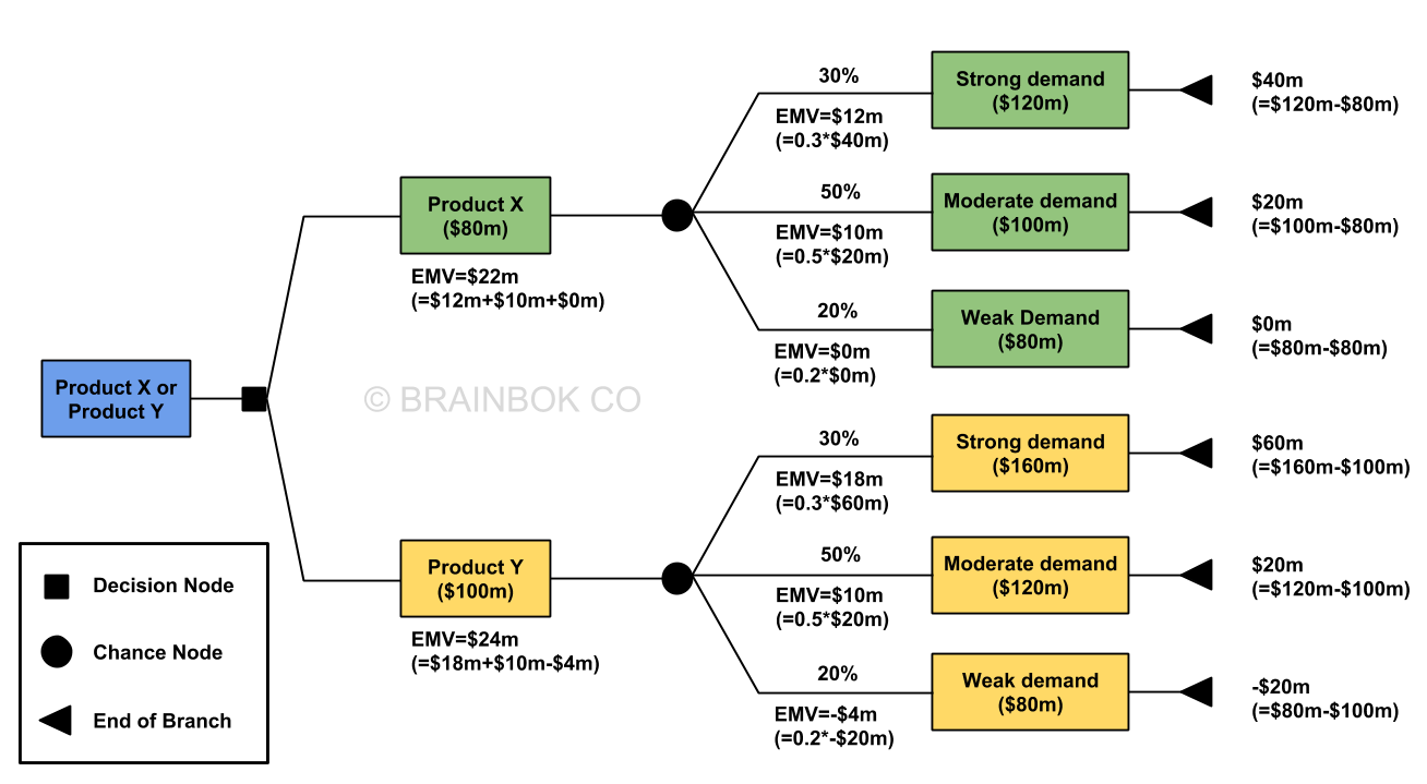
In summary, FitKit Inc. should go with Product Y and the EMV of their decision is $24m.
The final solution is shown in the image below.